What is calculus?

Calculus is the branch of mathematics that deals with the finding and properties of derivatives and integrals of functions, by methods originally based on the summation of infinitesimal differences. Gottfried Leibniz and Isaac Newton, 17th-century mathematicians, both invented calculus independently. Newton invented it first, but Leibniz created the notations that mathematicians use today.

The two types of calculus are;

1. Differentiation
2. Integration

Differential calculus determines the rate of change of a quantity. It examines the rates of change of slopes and curves. Integral calculus, by contrast, seeks to find the quantity where the rate of change is known. This branch concerns itself with the space or area under the curve. Integral calculus is used to figure the total size or value, such as lengths, areas, and volumes.

Why should we care?

 Before calculus was invented, all math was static It could only help calculate objects that were perfectly still. But the universe is constantly moving and changing. No objects—from the stars in space to subatomic particles or cells in the body—are always at rest. Indeed, just about everything in the universe is constantly moving. Calculus helped to determine how particles, stars, and matter move and change in real-time.

Calculus is used in a multitude of fields that you wouldn’t ordinarily think would make use of its concepts. Among them are physics, engineering, economics, and medicine.

Some of the concepts that use calculus include motion, electricity, heat, light, acoustics, and astronomy. Computer vision, artificial intelligence, robotics, video games, and even movies use calculus. It is also used to calculate the rates of radioactive decay, to predict birth and death rates, fluid flow, ship design, and even in the study of gravity

Differentiation

Differentiation by first principles

It is the origin of differentiation. We will illustrate differentiation by first principles by the below examples

Differentiating a linear function

A straight line has a constant gradient, or in other words, the rate of change of y with respect to x is a constant.

Example:

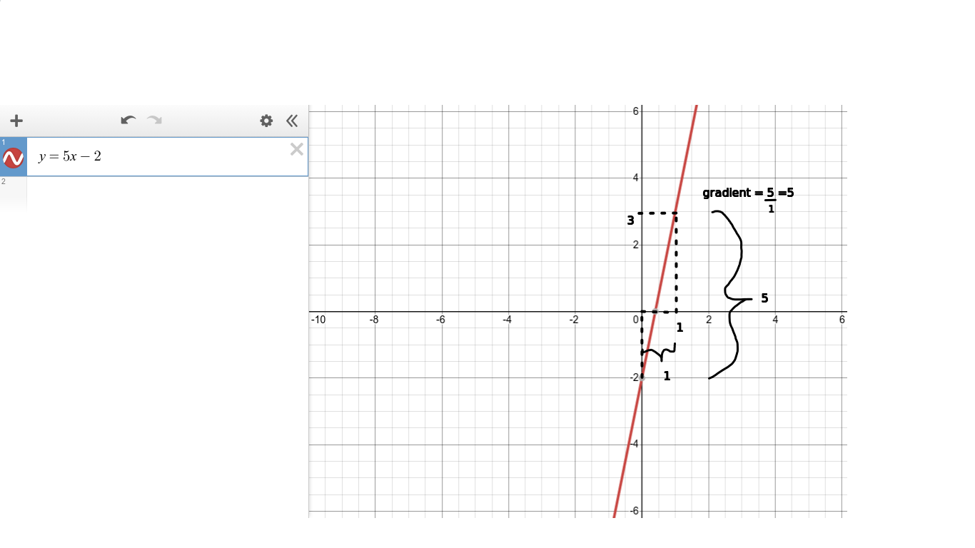
Consider the straight line y = 5x – 2 shown below:

Differentiation

A graph of the straight line y = 5x – 2.

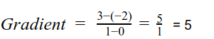
We can calculate the gradient of this line as follows. We take two points and calculate the change in y divided by the change in x.

When x changes from 0 to 1, y changes from −2 to 3, and so

No matter which pair of points we choose, the value of the gradient is always 5.

Values of the function y = 5x – 2 are shown below

x	-3	-2	-1	0	1	2	3
y	-17	-12	-7	-2	3	8	13

Look at the table of values and Look at the table of values and note that for every unit rise in x, y always increases by 5 units. We say that “the rate of change of y with respect to x is 5”.

Observe that the gradient of the straight line is the same as the rate of change of y with respect to x.

NOTE: For a straight line: the rate of change of y with respect to x is the same as the gradient of the line.

Differentiating a non-linear function

Now let’s look at differentiation from first principles of some simple curves.

For any curve, it is clear that if we choose two points and join them, this produces a straight line.

For different pairs of points, we will get a variety of lines with very different gradients. We illustrate below.

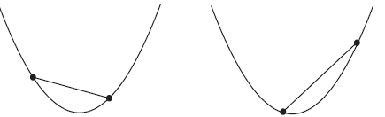
Joining different pairs of points on a curve produces lines with different gradients.

Example: Suppose we look at y = x².

x	-3	-2	-1	0	1	2	3
y	9	4	1	0	1	4	9

Note that as x increases by one unit, from −3 to −2, the value of y decreases from 9 to 4. It has been reduced by 5. But when x increases from −2 to −1, y decreases from 4 to 1. It has been reduced by 3. So even for a simple function like y = x², we see that y is not changing constantly with x. The rate of change of y with respect to x is not constant.

Calculating the rate of change at a point

We now explain how to calculate the rate of change at any point on a curve, y = f(x). It is defined to be the gradient of the tangent drawn at that point, as shown below

The rate of change at a point P is defined to be the gradient of the tangent at P.

NOTE: The gradient of a curve, y = f(x) at a given point is the gradient of the tangent at that point.

We use this definition to calculate the gradient at any particular point.

Consider the graph below, which shows a fixed point P on a curve. We also show a sequence of points Q1, Q2, . . . getting closer and closer to P. We see that the lines from P to each of the Qs get nearer and nearer to becoming a tangent at P as the Qs get nearer to P.

The lines through P and Q approach the tangent at P when Q is very close to P.

So if we calculate the gradient of one of these lines, and let the point Q approach the point P along the curve, then the gradient of the line should approach the gradient of the tangent at P, and hence the gradient of the curve.

Example :

 We shall perform the calculation for the curve y = x² at the point, P, where x = 3.

We shall calculate the gradient of the curve y = x² at the point P where x = 3.

The graph below shows the curve y = x² with the point P marked. We choose a nearby point Q and join P and Q with a straight line. We will choose Q so that it is quite close to P. Point R is vertically below Q, at the same height as point P, so that △PQR is right-angled.

The graph of y = x². P is the point (3, 9). Q is a nearby point.

Suppose we choose point Q so that PR = 0.1. The x coordinate of Q is then 3.1 and its y coordinate is 3.12. Knowing these values, we can calculate the change in y divided by the change in x and hence the gradient of the line PQ.

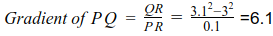
We can take the gradient of PQ as an approximation to the gradient of the tangent at P, and hence the rate of change of y with respect to x at the point P.

The gradient of PQ, will be a better approximation if we take Q closer to P. The table below shows the effect of reducing PR successively and recalculating the gradient.

PR	0.1	0.01	0.001	0.0001
QR	0.61	0.0601	0.006001	0.0006001
QR/PR	6.1	6.01	6.001	6.0001

The gradient of the line PQ, QR/PR seems to approach 6 as Q approaches P.

Observe that as Q gets closer to P the gradient of PQ seems to be getting nearer and nearer to 6.

We will now repeat the calculation for a general point, P, with has coordinates (x, y).

The graph of y = x². P is the point (x, y). Q is a nearby point.

Point Q is chosen to be close to P on the curve. The x coordinate of Q is x + dx where dx is the symbol we use for a small change or small increment in x. The corresponding change in y is written as dy. So the coordinates of Q are (x + dx, y + dy).

Because we are considering the graph of y = x², we know that y + dy = (x + dx)².

y +δy = (x + δx)² = x² = 2x(δx)+ (δx)²

But y=x² and so, δy =2x(δx)+ (δx)²

So the gradient of PQ is

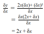
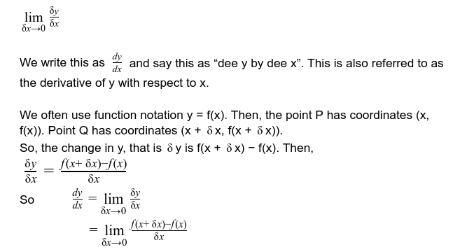
As we let δx become zero we are left with just 2x, and this is the formula for the gradient of the tangent at P. We have a concise way of expressing the fact that we are letting δx approach zero. We write;

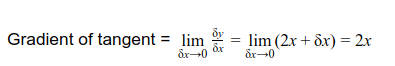
‘lim’ stands for ‘limit’ and, we say that the limit as dx tends to zero of 2x+dx is 2x. Note that when x has the value 3, 2x has the value 6, and so this general result agrees with the earlier result when we calculated the gradient at the point P(3, 9).

We can do this calculation in the same way for lots of curves. We have a special symbol for the phrase

Integration

Isaac Newton and Gottfried Wilhelm Leibniz formulated the principles of integration independently by thinking of an integral as an infinite sum of rectangles of infinitesimal width.

Antidifferentiation is the process of obtaining y when dy/dx is known, while the process of finding an area under a curve is known as integration. There is a remarkable theorem due to Newton and Leibniz which states “integration is essentially the same as antidifferentiation”. It is known as the Fundamental Theorem of Calculus.

Therefore, we will not use the term differentiation. So from now on, we will only talk about integration.

Indefinite integrals

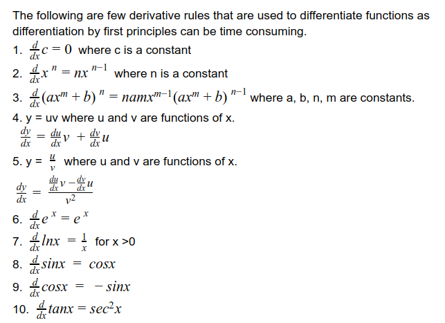
Using the  Fundamental Theorem of Calculus, we can get the following rules.

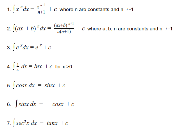
Now, I’m sure most of you are wondering, “What is this c ?”. Well, c is an arbitrary constant. We add it so that our answer represents all the possible solutions for the integral. What do I mean by all the possible solutions?

The diagram below demonstrates this.

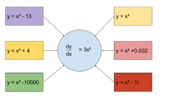
Since the derivative of all these functions is 3x², it follows that the solution for the integral of 3x² can be all of these functions. 

NOTE: 

There are infinitely many functions whose derivative is 3x² but only a few are shown here. Hence there are infinitely many functions that can be the solution for the integral of 3x². But they are all represented by y = x³ + c. This is known as the general solution. 

The function which is the solution to the integral is called the primitive function. If more information about the primitive function is known, we can find a specific function. (For example, coordinates of a point through which the graph of the primitive function passes through)

Definite integrals

Here we will be applying limits to the integral. Given below is an example:

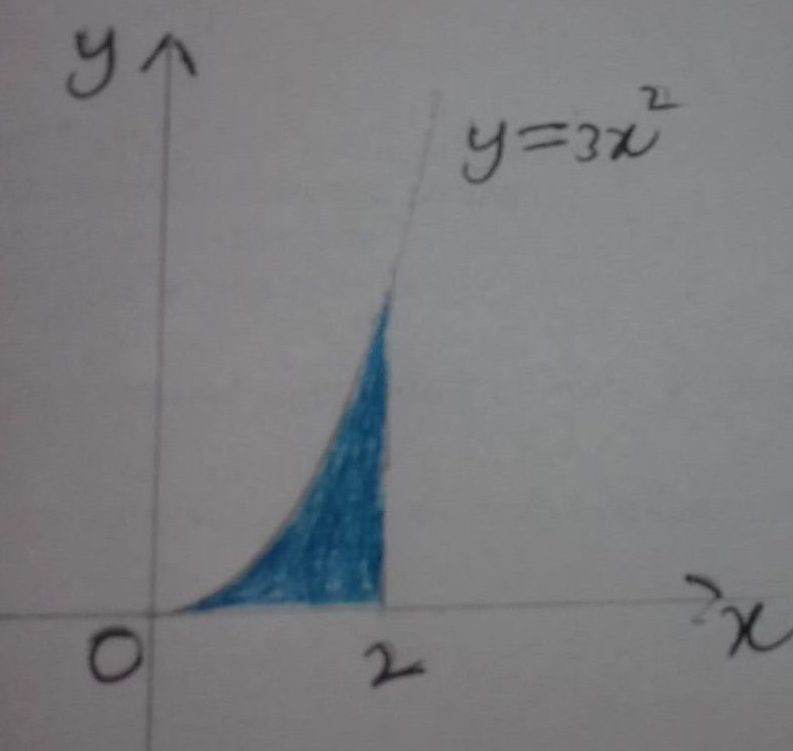
y=3x²  Find the area under the graph from x=0 to x=2

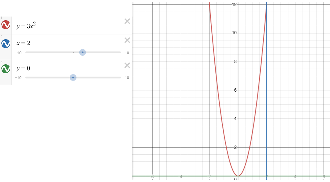
So now the question is, how can we find the area enclosed by the coloured lines. The integral below does the job;

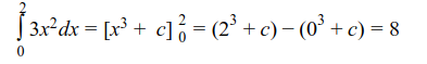
There are several interesting things to note here;

1. The answer is a number that represents an area
2. The arbitrary constant gets cancelled
3. The rules used for indefinite integrals are applied

Because of the 2nd point, we don’t include c in our work when solving a definite integral.

Now I’m sure most of you are wondering, “What black magic is this? Does it even give the correct value?”. Well, you can check it on your own using an accurate sketch of the graph.

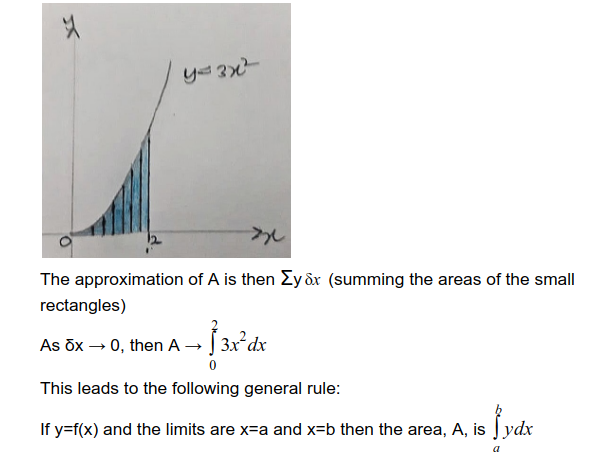
To explain how it works consider the area bounded by the curve y=3x², the x-axis and the lines x=0 and x=2

The area, A, of the region can be approximated by a series of rectangular strips of thickness δx (meaning a small increase in x) and the height y (meaning the height of the function).

If the required area is below the x-axis, then the integral evaluates to a negative value. So when part of the total area is below the x-axis while the other is above the x-axis you have to evaluate each area separately.

Also, you can find the area enclosed by a curve and the y-axis too. In this scenario, the function is written in terms of y with x as the subject. The limits are values of y and the function is integrated with respect to y.

The general rule:

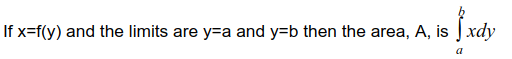
In this case, if the required area is to the left of the y-axis, then the integral evaluates to a negative value. If it is to the right of the y-axis, then you get a positive value. 

In summary, calculus allows us to make models for moving objects and make predictions. Calculus can be used to find rates of change of a quantity(using differentiation) or find a quantity when its rate of change is known(using integration). Thanks to Calculus, math became dynamic. I hope you became inspired to learn more about Calculus. Have a nice day!

INESH PALIHAPITIYA

Citations and Resources:

http://www-math.mit.edu/~djk/calculus_beginners/chapter00/section02.html

https://www.thoughtco.com/definition-of-calculus-2311607

https://revisionmaths.com/advanced-level-maths-revision/pure-maths/calculus/differentiation-first-principles#:~:text=This%20section%20looks%20at%20calculus%20and%20differentiation%20from%20first%20principles.&text=A%20straight%20line%20has%20a,to%20x%20is%20a%20constant.&text=A%20graph%20of%20the%20straight%20line%20y%20%3D%203x%20%2B%202.

https://www.desmos.com/calculator

Cambridge International AS & A Level Mathematics: Pure Mathematics 1 Coursebook (Publisher: Cambridge University Press Series Editor: Julian Gilbey Author: Sue Pemberton ISBN: 9781108407144)

Cambridge International AS & A Level Mathematics: Pure Mathematics 2 & 3 Coursebook (Publisher: Cambridge University Press Series Editor: Julian Gilbey Authors: Sue Pemberton, Julianne Hughes ISBN: 9781108407199)